Skill 7: Conditional formatting
Excel can automatically format cells depending on their values. This is called “conditional formatting”.
Conditional formatting is useful when you have a lot of data and want visual cues to examine the data further, such as a month where payments are above a certain amount.
In this lesson we’ll explore conditional formatting and practice applying it to some sample data. To get you started, download and open the sample spreadsheet below.
- XYZ sample spreadsheet 3
In this lesson we will learn how to:
- Highlight top 10 values
- Highlight specific text
- Highlight values less than X
- Highlight empty cells
- Remove conditional formatting
The video below will show you through these tasks, and they’re also explained in writing underneath.
Highlight top 10 values
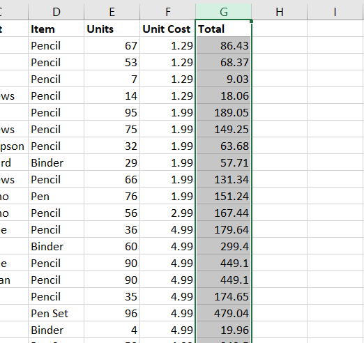
Let’s imagine we want to know the highest numbers in the “Total” column. We’d rather not sort the column, so let’s use formatting to highlight the top 10 values.
First, highlight the column you’d like to format. In our example, this is column G. Click on the G to highlight the entire column.
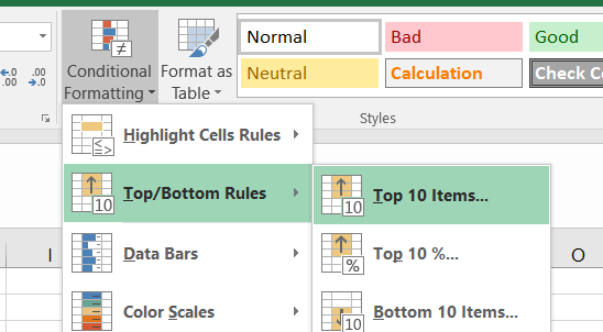
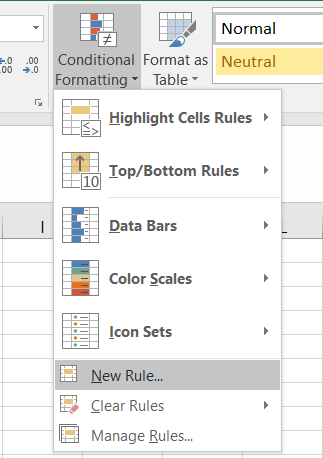
In the “Home” menu ribbon, click Conditional Formatting > Top/Bottom Rules > Top 10 Items.
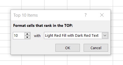
In the box that appears, you will see that you can adjust the number (so that it’s not the top 10, but the top anything) and the formatting. For this example, let’s leave it on the default values:
If you scroll down, you will see the top 10 values have been highlighted in red.
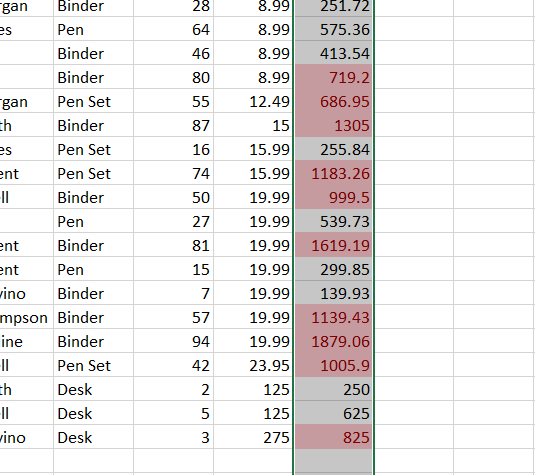
Practice point: Use conditional formatting to highlight the top 10 values in column G.
Highlight specific text
Using the same technique, we can highlight specific text. For example, let’s say we want to highlight every time the word “Pencil” appears in column D.
Click on the letter D to highlight the entire column. Then go to Conditional Formatting > Highlight Cell Rules > Text that Contains.
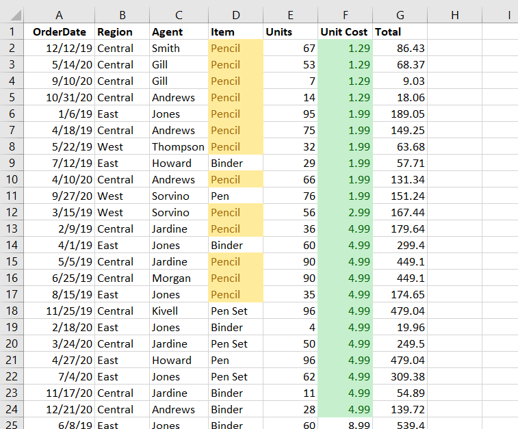
Type “Pencil” in the box, and select “Yellow Fill with Dark Yellow Text”.
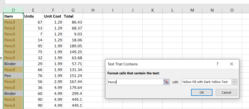
Your column now highlights every time the word “Pencil” appears in column D.
Practice point: Highlight the cells containing the word “Pencil” in column D.
Highlight values less than X
We’ve already learned how to highlight the top 10 values in a list, or specific words. Now we will learn how to highlight values under a certain value. To practice this, we’ll use column F.
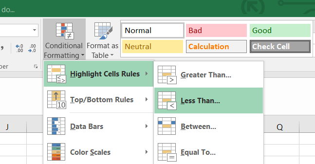
Click on the letter F to highlight the entire column. Then go to Conditional Formatting > Highlight Cell Rules > Less Than.
Type 5 in the box, and choose “Green Fill with Dark Green Text”, then Ok.
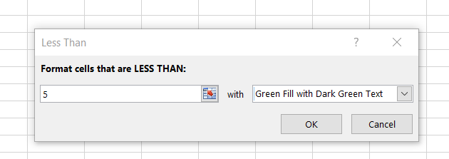
This will make every value in column F that is under 5, turn green.
This technique is very useful for finding figures under a certain value. But we can also format cells that are equal to a certain amount, or over a certain amount. Explore the menu Conditional Formatting > Highlight Cell Rules.
Practice point: Use the menu Conditional Formatting > Highlight Cell Rules to highlight numbers in column F that equal 23.95.
Highlight empty cells
It can be useful to highlight empty cells. You might use this when you’ve been entering some data and want to highlight any cells you might have missed.
First, let’s imagine we’ve missed entering data in cells F7, F12 and F22. We’ve going to click on each of them in turn, and press the Backspace or Del key to remove the data.
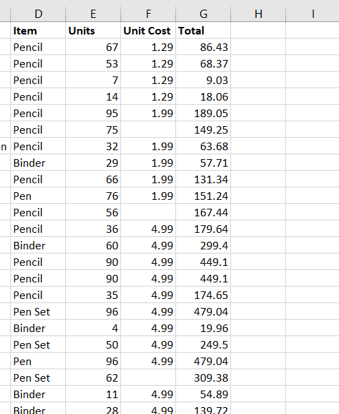
Practice point: Remove data from cells F7, F12 and F22.
Click on column F to highlight the column (click on the letter F to highlight the whole column). Go to Conditional Formatting > New rule.
In the box that appears, choose “Format only cells that contain”
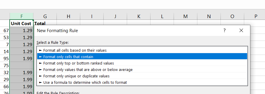
In the bottom part of the box, change “Cell value” to “Blanks”.
Next, click Format > Fill > click on the yellow color > Ok.
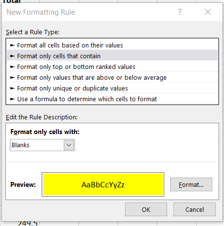
As you click on Ok, the blank cells will turn yellow. It should look like this:
![]()
Highlighted blank cells
Edit / remove conditional formatting
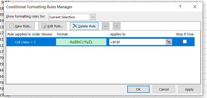
To edit/remove conditional formatting:
- Highlight the column, row or cell where the conditional formatting is displaying
- Go to Conditional Formatting > Manage Rules. This will show you all the current rules being applied. Here you can edit or remove them.

Great work!
Now that you know how to do conditional formatting, your Excel skills are becoming more and more useful. If you’ve completed all the practice points in this lesson, you’ve done some great work!
Before moving on, have a look at the checklist below. You should be able to do all these things now. If not, go back through this lesson and practice some more. When you feel comfortable that you’ve got these things sorted, tick them off and move on to the next lesson.
[checklist_in_post]- Highlight top 10 values
- Highlight specific text
- Highlight values less than X
- Highlight empty cells
- Remove conditional formatting